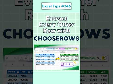
Excel: extract every other row with CHOOSEROWS

Key insights

• Use SEQUENCE to generate row positions, then pass them to CHOOSEROWS.
• ROUNDUP includes the last odd-positioned row when the source has an odd number of rows.
• The row indexes refer to positions within the selected array, not worksheet row numbers.
• The results spill into neighboring cells, so the output area must be clear.
• CHOOSEROWS selects by position; use FILTER when rows must meet a condition.

Excel’s CHOOSEROWS function can extract alternating rows from a range or table, returning the selected records together as a dynamic array. This is useful for spreadsheet users who want every other record without adding a helper column or manually copying rows. Alan Murray (Computergaga) demonstrates the task in a YouTube Short.

What it does

CHOOSEROWS returns complete rows from an array based on row positions you provide. Combined with SEQUENCE, it can generate those positions automatically: 1, 3, 5, and so on. The formula returns all the columns for each selected row, keeping each record intact.

For example, this formula extracts every other row from the range A2:D20: =CHOOSEROWS(A2:D20,SEQUENCE(ROUNDUP(ROWS(A2:D20)/2,0),,1,2)). It counts the rows in the source, creates a sequence of odd positions, and passes those positions to CHOOSEROWS. The same pattern can work with a table reference such as SalesData.

Who it is for and what you need

This technique is for people working with Excel ranges or tables who need a non-contiguous selection of records. The material does not specify a required license, Excel version, platform, or rollout status, so check whether CHOOSEROWS and dynamic arrays are supported in your Excel environment.

The output is a spilling array: Excel fills the cells around the formula with the returned rows. Keep the spill area clear, or the result cannot expand there. The source range should include the data rows you want to evaluate.

For more Excel guidance, see our Excel coverage.

How it works

1. Choose the source range or table, such as A2:D20.
2. Enter the formula =CHOOSEROWS(A2:D20,SEQUENCE(ROUNDUP(ROWS(A2:D20)/2,0),,1,2)) in an empty output area.
3. Press Enter and let the returned rows spill into adjacent cells.

To return even-positioned rows instead, use =CHOOSEROWS(A2:D20,SEQUENCE(INT(ROWS(A2:D20)/2),,2,2)). Change the sequence start and step to select a different pattern; for example, a step of 3 selects positions 1, 4, 7, and so on.

Limitations and open questions

CHOOSEROWS selects by position, not by a value or other condition. For conditional selection, FILTER may be a better fit. Row position zero or a position beyond the source array produces a #VALUE! error, and a blocked spill area prevents the result from expanding.

Older approaches may use helper columns with MOD or ISEVEN, or combinations of INDEX, ROW, and MOD. The supplied material does not establish which Excel versions support this formula or describe a specific alternative for versions without it. It also provides no official Microsoft source for compatibility or licensing details.

Sources

• Alan Murray (Computergaga) YouTube Short

Frequently asked questions

How do I extract every other row in Excel?

Use CHOOSEROWS with SEQUENCE to generate odd row positions: =CHOOSEROWS(A2:D20,SEQUENCE(ROUNDUP(ROWS(A2:D20)/2,0),,1,2)).

Can CHOOSEROWS return even-positioned rows?

Yes. Start the sequence at 2 and use a step of 2: =CHOOSEROWS(A2:D20,SEQUENCE(INT(ROWS(A2:D20)/2),,2,2)).

What do I need to use CHOOSEROWS?

The material describes using CHOOSEROWS with dynamic arrays, but does not state which Excel versions, licenses, platforms, or regions support it.

Why does Excel show an error for CHOOSEROWS?

A row index of zero or one that exceeds the source array's row count produces #VALUE!. The output also needs an unobstructed spill area.