Excel financial modeling: checks and scenario analysis
Co-Founder at Career Principles | Microsoft MVP
Use Excel’s Watch Window, model checks, Goal Seek and Data Tables to monitor results and test financial assumptions.
Key insights
- Watch Window keeps selected results visible while you change inputs on another worksheet.
- Use IF checks to flag negative cash and a TRUE/FALSE comparison to test whether a balance sheet balances.
- EOMONTH and EDATE can link model dates to a start date and fill periods across a row.
- Data Validation can restrict a scenario selector to options such as Base, Upside and Downside.
- Goal Seek finds an input value that produces a target result; a Data Table compares two changing inputs.
Excel’s financial modeling tools can help you monitor outputs, catch input errors and test scenarios without repeatedly navigating between worksheets. They are useful for analysts and other Excel users who build or review forecasts with changing assumptions. Kenji Farré (Kenji Explains) [MVP] demonstrates these techniques in a YouTube video.
What it does
These techniques focus on making a financial model easier to use and inspect rather than replacing its underlying calculations. The Watch Window tracks selected cells as you change assumptions elsewhere, while Freeze Panes and grouped rows or columns make larger workbooks easier to navigate.
Model checks can flag conditions such as negative cash or a balance sheet that does not balance. Dynamic dates and dropdowns reduce repetitive edits and typos. For analysis, Goal Seek works backward from a target result, while a two-variable Data Table shows how an output changes across combinations of assumptions.
Who it is for and what you need
The techniques are aimed at people working with financial models in Excel, including analysts who change inputs and review outputs across worksheets. They start with an existing workbook containing model assumptions, calculations and results; the examples use annual and monthly figures, scenario names, cash balances and profit.
The steps use Excel features found on the Formulas, View, Data and File tabs. A few steps depend on the model being set up appropriately: Goal Seek needs a target result cell and a cell it can change, and a Data Table needs an output linked to the model plus input cells corresponding to its row and column assumptions.
How it works
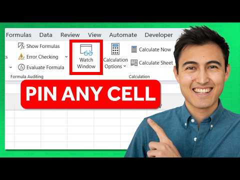
- Track important outputs. Select a result such as net profit or closing cash, then choose Formulas > Watch Window. Keep the Watch Window open while changing assumptions on another worksheet; it updates the displayed values. You can add more cells, including cells on other tabs.
- Keep headings visible. On the View tab, use Freeze Panes. To freeze both rows and columns, select the cell below and to the right of the area you want to keep visible, then apply the command. The selected position matters: freezing a column alone does not also freeze the rows.
- Show hidden detail as a group. Select the rows or columns to group and choose Data > Group. Excel adds outline controls so users can collapse and expand sections. The demonstrated shortcut for grouping is Shift + Alt + Right Arrow.
- Add simple model checks. An IF formula can display “Check” when a cash figure is below zero and “OK” otherwise. To test whether assets and liabilities match, compare the two cells; the equality test returns TRUE or FALSE. An IF statement can also display a label for that result.
- Link dates and restrict scenario names. Use EOMONTH with the model start date and zero months to return the month-end date. Use EDATE to move forward by a chosen number of months, then fill the formula across. For a scenario selector, choose Data > Data Validation, set the allowed values to a List, and enter or select the permitted names.
- Find a target or compare two assumptions. Choose Data > What-If Analysis > Goal Seek. Set the result cell, enter the target value, and select the input cell Excel should change. For a two-variable sensitivity table, link its output corner to the model result, select the table, then choose What-If Analysis > Data Table and assign the row and column input cells to the corresponding assumptions.
A reusable formatting guide can also standardize colors and number formats. The demonstration saves a workbook template as an .xltx file named “Book” in the Excel XLSTART folder, so it opens with new workbooks. A format painter can copy a custom number format, such as displaying a negative percentage in parentheses.
Limitations and alternatives
These tools do not substitute for checking the model’s logic. A comparison that returns TRUE or FALSE only tests whether the two referenced cells are equal; it does not verify every part of a balance sheet or explain a mismatch. Likewise, an “OK” cash check depends on pointing the formula at the intended cash value and testing the condition the model needs.
Goal Seek changes one input cell to reach one target in a result cell. When the question involves two assumptions at once, a Data Table is the demonstrated alternative. Set its row and column input cells carefully: swapping them can make the sensitivity grid represent the wrong assumptions. Freeze Panes also depends on selecting the correct split point before applying it.
Sources
Frequently asked questions
How do I keep Excel results visible while changing inputs on another sheet?
Select the result cells and choose Formulas > Watch Window. The selected values remain visible and update as you change inputs, including on another worksheet.
How do I use Goal Seek for a financial model?
Choose Data > What-If Analysis > Goal Seek. Set the result cell, enter the target value, and select the input cell Excel should change to reach it.
How do I create a two-variable sensitivity table in Excel?
Link the table’s output corner to the model result, select the table, and choose Data > What-If Analysis > Data Table. Assign the row and column input cells to the matching assumptions.
How can I prevent typos in an Excel scenario selector?
Use Data > Data Validation and select List. Enter or select the allowed scenario names so the cell is restricted to those options.